Introduction
The Atari Learning Environment (ALE) has been a foundational benchmark for reinforcement learning for over a decade, serving as the training ground for millions of agents and many of the field's most influential algorithms. However most of this progress has occurred in simulation, where environments are fast, parallelizable, and perfectly synchronized with the agent.
In this work, we ask if these methods still work when the Atari environment is embodied in the physical world? Specifically, we study reinforcement learning on a real robot that plays Atari games on an actual console, operating under real-time constraints, with hardware limitations, and limited compute. Our investigation is motivated by RL efforts at Sutton's AMII lab and KeenAGI who designed and open-sourced their robot and learning framework - the Physical Atari benchmark.
Quick Review of RL (click to expand)
If you are unfamiliar with RL, we highly recommend these resources for getting started: ARENA 3.0, Hugging Face Deep RL Course, and Sutton & Barto's RL Book.
Key Terms
- Rewards are positive signals that are given to the agent when it does something that we want it to. In Ms. Pacman rewards are given for eating pellets, eating ghosts, and eating cherries.
- Actions are taken by the agent to move around or perform tasks in an environment. In Ms. Pacman the valid actions are UP, DOWN, LEFT, RIGHT.
- States are the world that an agent exists within, while observations are a subset of the state that the agent can use to take actions.
- A policy is the agent's decision making framework for taking specific actions. Given a state, the policy decides which action to execute. Some policies are neural networks, others are argmax().
Bellman Equation
The Bellman Equation tells us how “valuable” it is to be in a given state. It is the sum of expected future rewards from a state given that we take the maximal action in each future state, and account for environment randomness.
Temporal Difference Learning
Knowing the true value of a state is very difficult, because it requires perfectly exploring the entire recursive tree of the bellman equation above. Exploring the environment in this manner is usually computationally impossible, so our deep networks must learn to estimate the values from experiences it has had. Temporal difference learning allows us to update our estimate of a state V given future rewards we have received!
The equation above describes how we update our estimate V(S_t) based on just a single step forward in the environment V(S_t+1) called TD(0). Sutton extended this algorithm further to TD(λ) which updates the estimate based on rewards from all future rewards received.
These estimates for the value function for given states are used in computing the loss for our deep neural networks.
Deep Q-learning
We often rewrite the bellman equation for Q-learning as conditioned on a specific action. This is fundamentally the same equation, except the inputs are both the state and action taken.
Q-learning aims to maximize the objective of: “can a neural network learn to predict the value of taking a specific action given a certain state of the environment?” In discrete environments like Ms. Pacman, the network might be learning to produce the values of taking each of the actions simultaneously, for example Q(s,[UP,DOWN,LEFT,RIGHT]) = [8.4, 7.2, 0.6, 5.2]. The policy decides to take the maximum value action from this list.
Policy Gradient
Policy gradient methods employ a different strategy for selecting actions. Instead of producing Q values, policy gradient methods have an objective of “can a neural network learn to predict a distribution over actions given a certain state of the environment?”. In Ms. Pacman, this might look something like π(s) = [UP=25%, DOWN=8%, LEFT=60%, RIGHT=7%]. The policy will sample from this distribution instead of simply taking the maximum value. This is quite helpful in environments that are stochastic (like poker), where always taking the maximum value action might lead to poor performance.
Advantage Estimation
When an agent chooses an action in a state, what we actually care about is how much better or worse that action is compared to the average action the policy would normally take in that state. This quantity is called the advantage:
The advantage is measured by taking action-value Q(s,a) and subtracting the state-value V(s). This tells us how much better a specific action is with respect to the current policy distribution. By subtracting out V(s), we are also reducing variance without introducing bias because we eliminate the part of the signal that has nothing to do with which action we chose.
In policy gradient methods, the loss uses this advantage term to decide how the policy should change. A positive advantage increases the probability of an action, a negative advantage decreases it, and a zero advantage leaves the policy unchanged. This ensures that the gradient update is driven by improvements over the policy's baseline behavior rather than raw returns.
This variance reduction is critical in long-horizon environments like Ms. Pacman where rewards are sparse, delayed, and stochastic. It stabilizes training and makes each update more sample-efficient. Actor-Critic is a training method where both a value network and a policy network are trained simultaneously to produce the advantages.
Our goals were three-fold:
- Understand the difference between training agents in simulation and in the real-world
- Benchmark existing approaches on real hardware
- Develop intuition for which approaches are best suited to robots: value-based or policy gradient methods
Challenges with real time robot RL
Real-time robot reinforcement learning faces three structural constraints that do not exist in simulation-first settings: robots must learn at the pace of real-time, they are hardware bound, and environments in the real-world are not turn-taking.
1. Time Bound
Physical robots operate in the real-world. This means that robots can't step through environments faster than real-time, which places a hard upper bound on the amount of data available for learning. Our system observes the environment at the camera's framerate of 60fps, which means over a period of 12 hours it can maximally collect 2.5m frames. Not all of these frames are useful (game resets, frame skips [4], etc), and we measured something closer to 500k useful observations. Conversely, a simulator on the same machine can step through the Ms. Pacman environment at around 500fps, producing over 20 million transitions in the same time period. The gap between simulated and real agents is that real-agents must find more efficient ways to process observations.
2. Hardware Bound
Robots are bound by the constraints of physical hardware. Building more robots is time and cost intensive where parallelizing simulated agents is relatively easy.
In our experiments data collection was limited to a single robot controller, a single Atari console, and a single GPU (RTX 5090). This constraint extends beyond the lab; most commercial/industrial deployments operate on the order of hundreds to thousands of robots, orders of magnitude fewer than the number of agents routinely used in simulation.
The lack of parallel actors fundamentally alters the learning dynamics. Without multiple environments running concurrently, on-policy trajectories are sequential and highly temporally correlated, removing a key mechanism used in simulation to stabilize updates and reduce variance.
Our robot was subject to hardware wear and tear and environmental variation. There were many training runs where 3D printed parts snapped, bolts came loose, or the sun set before we had a chance to turn the lights on and performance diverged. Managing these ever-changing variables is something that RL practitioners must do every day with robots.
3. Environment Bound
In typical reinforcement learning benchmarks, environments are turn-taking: the environment waits for the agent to complete inference, select an action, and even perform gradient updates before advancing to the next state. This assumption does not hold in the real world. The real-world is ever changing, and agents must be adaptive and flexible enough to react to those changes as they occur.
The lack of turn-taking is a key differentiator between RL environments that operate in simulation and those that operate in the physical world. For example, a Ms. Pacman agent that takes one minute to perform a network update will achieve the same score as an agent that takes one millisecond in simulation, because the environment steps in synchrony with the agent. On a robot, this agent would die every time because the ghosts would catch up to it.
In reality, the robot does not have the leisure of infinite time to perform inference, take actions, and compute gradient update steps. Computational efficiency of both inference and learning is critical to ensure that a physical robot is not discarding useful experiences or diverging into poor states because it cannot update its network fast enough. In this work we explore methods that work around this constraint.
Robotroller Build Details
The primary build instructions and physical setup details can be found here.
tl;dr for those who just want the highlights:
- Controls: Robotroller (robot controller) attaches to an Atari Joystick enabling clicking of the fire button and full joystick control via 3 servo motors
- Perception: High resolution web camera points at monitor where the Atari game is visible.
- Frame is detected and centered via 4 april tags at the corners of the game area.
- Rewards are assigned via a custom score-detection CNN model that detects when the score of the game increments.
- Materials: Robot is 3D printed with PLA about .25kg of material + motors/controller
- Compute: Desktop GPU with RTX 5090
Experiments
| Algorithm | Peak Mean Reward | Final Mean Reward | Top Score | Frames |
|---|---|---|---|---|
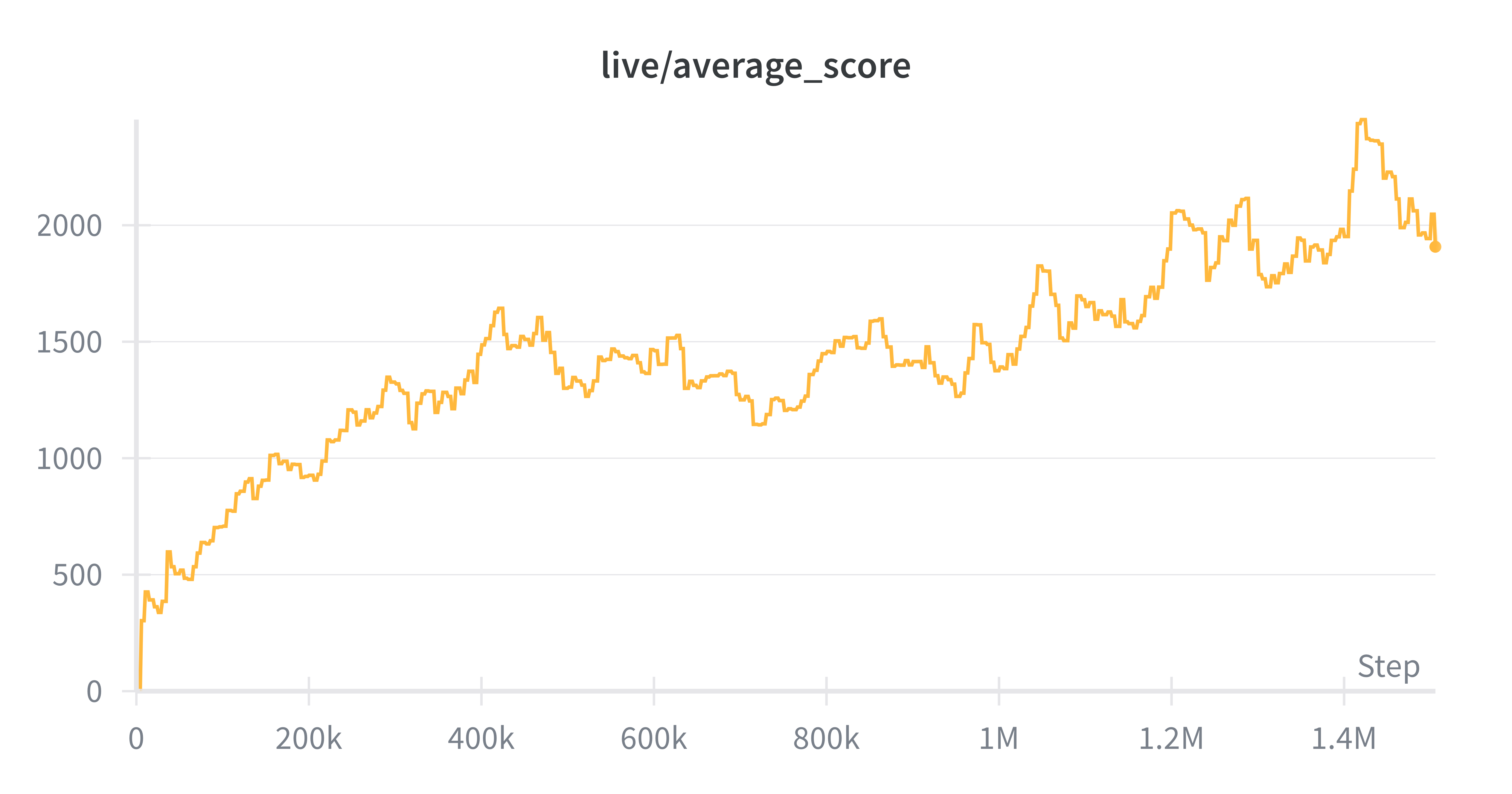
| Delay Target | 2463 | 2047 | 4420 | 1.5m |
| SAC | 1176 | 1091 | 2330 | 1.5m |
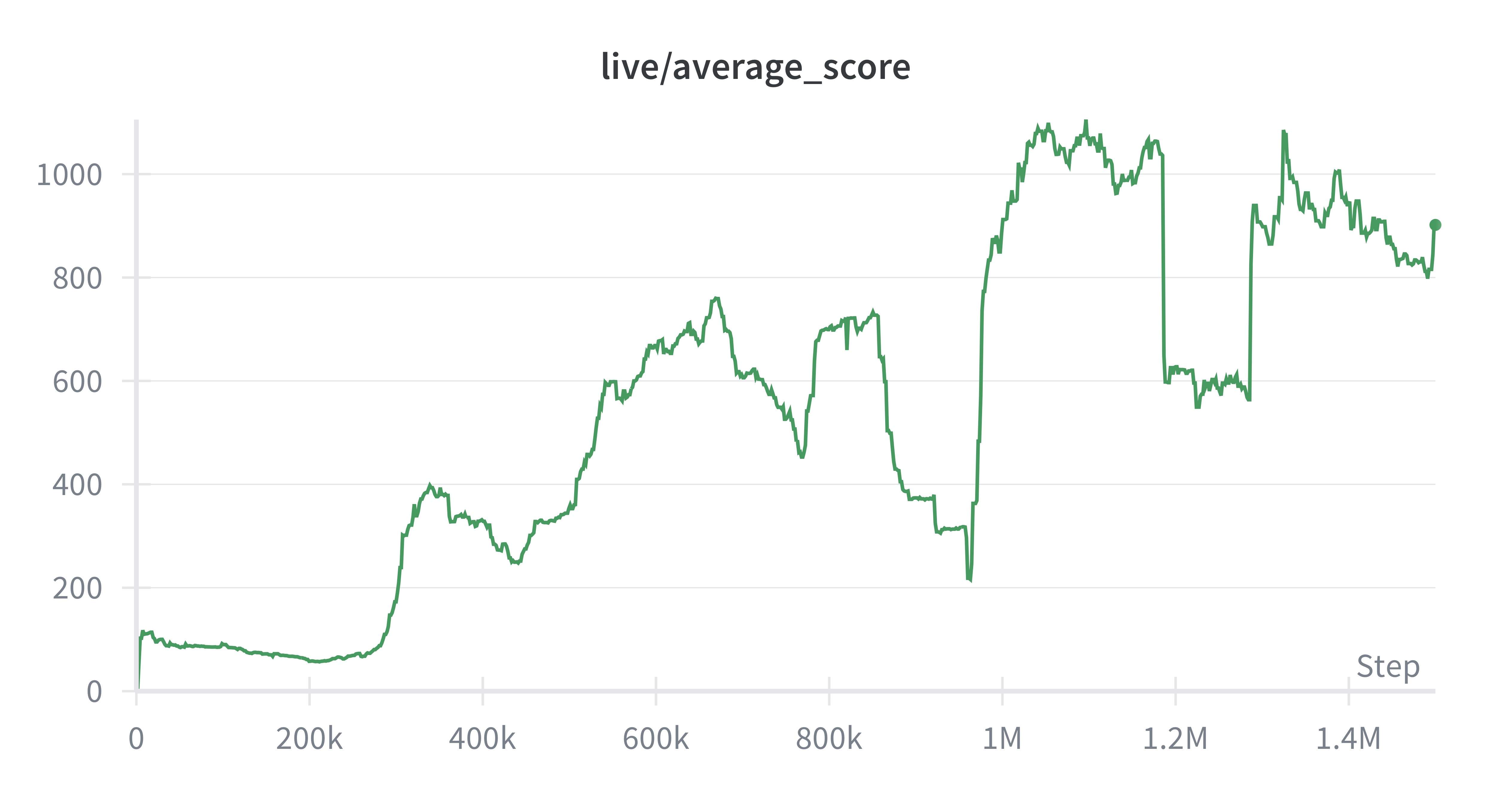
| Rainbow DQN | 1085 | 902 | 2950 | 1.5m |
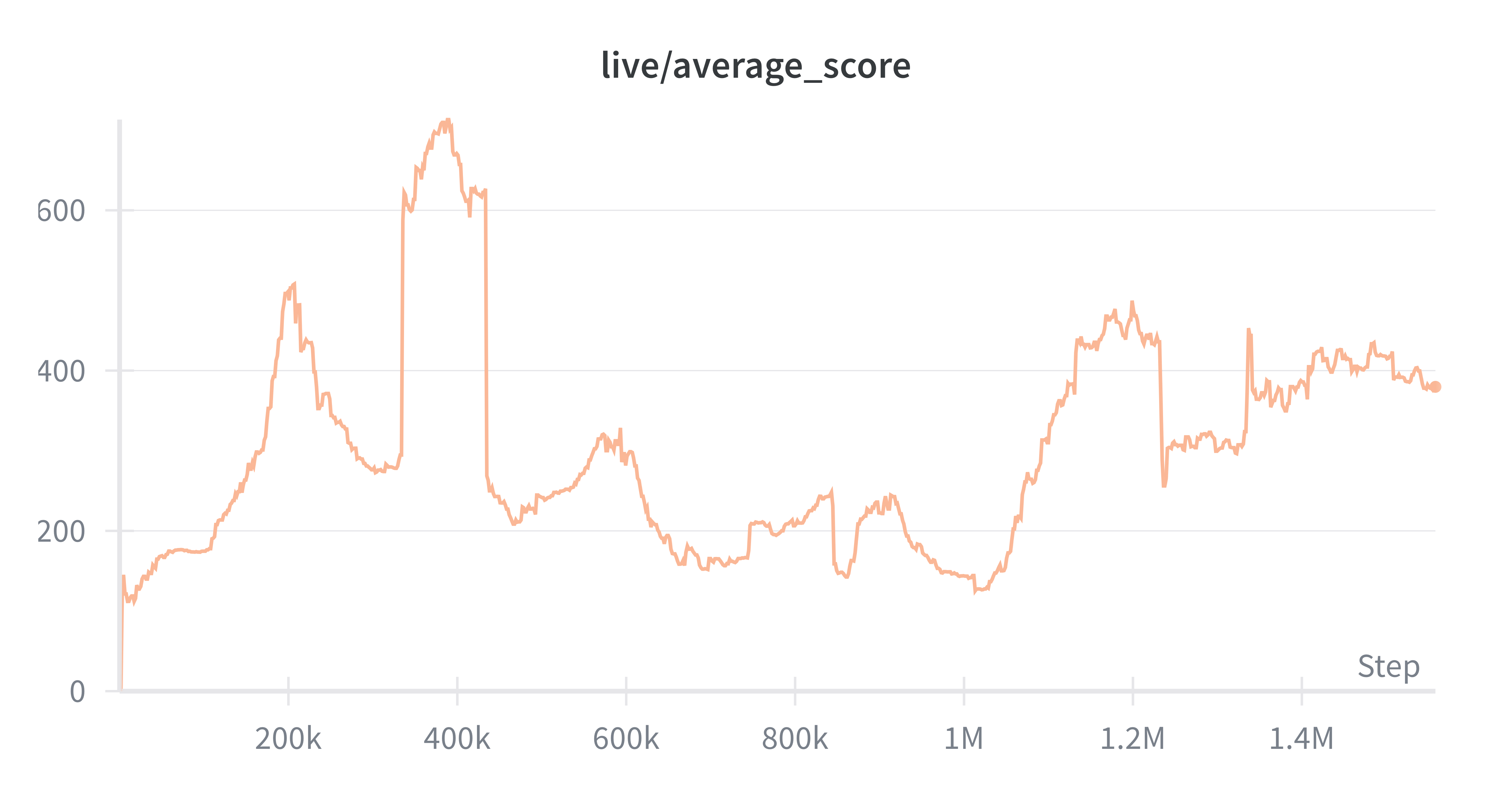
| PPO | 670 | 379 | 3180 | 1.5m |
Delay Target
Rainbow DQN
PPO
SAC
In this section we will cover the algorithms tested on the Physical Atari. Each agent was trained over 1.5M environment steps (~8hrs). Ms. Pacman was chosen for its semi-exploratory nature + dense rewards.
Rainbow DQN
Rainbow DQN is an enhanced version of Vanilla DQN. It combines 6 independent improvements to improve sample-efficiency and performance.
Key Features
Distributional RL
Instead of predicting a single expected value Q(s,a), Rainbow predicts a distribution over possible returns for each action. This is the core difference between Rainbow DQN and Vanilla DQN.
Greedy action selection uses the mean of the predicted distribution.
Training then matches the predicted distribution to a target distribution (typically via cross-entropy / KL).
Double DQN
In Vanilla DQN, the target network chooses the next action and uses it for evaluation in the loss. In Double DQN the online network selects this action:
By using the online network to select actions, the bias to the bootstrapped value decreases.
Prioritized Replay
Vanilla DQN samples uniformly, while Rainbow DQN prioritizes transitions where the model's current prediction distribution disagrees most with its target distribution.
Sampling is done probabilistically based on priority (learning loss). If a sample results in a larger priority it has a higher probability of being sampled.
Dueling Networks
In most states, the choice of action has little influence on the outcome compared to the value of simply being in that state. For example, when Ms. Pac-Man is in a large open area with no nearby ghosts, most actions keep her safe, so the expected return is dominated by being in a safe state rather than by which direction she moves.
Dueling networks exploit this by decomposing the Q-function into two components: a value function V(s), which captures how good a state is, and an advantage function A(s, a), which measures how much better a given action is relative to the average action in that state. These two terms are then recombined to produce Q(s, a).
Architecturally, this corresponds to a shared CNN backbone followed by two separate heads: one estimating state value and the other estimating action advantages.
Multi-step returns
Vanilla DQN uses a single step for bootstrapping the target return, Rainbow uses multi-step return to bootstrap the returns in the target distribution.
Multi-step returns push learning signal back faster (more “credit assignment per update”), often improving early learning and sample efficiency.
Noisy Nets
Noisy Nets are a replacement for epsilon-greedy in DQN. Epsilon-greedy injects randomness at the action selection level, whereas Noisy Nets inject randomness into the Q-function parameters:
where , are random variables and is an elementwise product.
The network learns the noisy weights and biases which determine how much noise needs to be injected in learning (will inject more if exploration is required), making exploration trainable.
Observations
Rainbow DQN showed strong learning on the physical robot setup, which is consistent with the fact that value-based Q-learning methods tend to perform well in discrete action spaces (and Atari games). What surprised us, however, was how readily the learned policy executed aggressive, high-commitment maneuvers, such as quickly repositioning to avoid ghosts, in a way that resembles skilled human play. In simulation this kind of behavior is expected because actions can be applied effectively instantaneously and with minimal input uncertainty. On the physical system, by contrast, the camera-based control loop and controller latency introduce delays between issuing a command and seeing its effect on-screen, so we would have expected the policy to behave more conservatively. The fact that Rainbow still learned these decisive evasive actions suggests it was able to internalize the delayed dynamics of the real control interface and plan effectively despite the added latency.
Delay Target
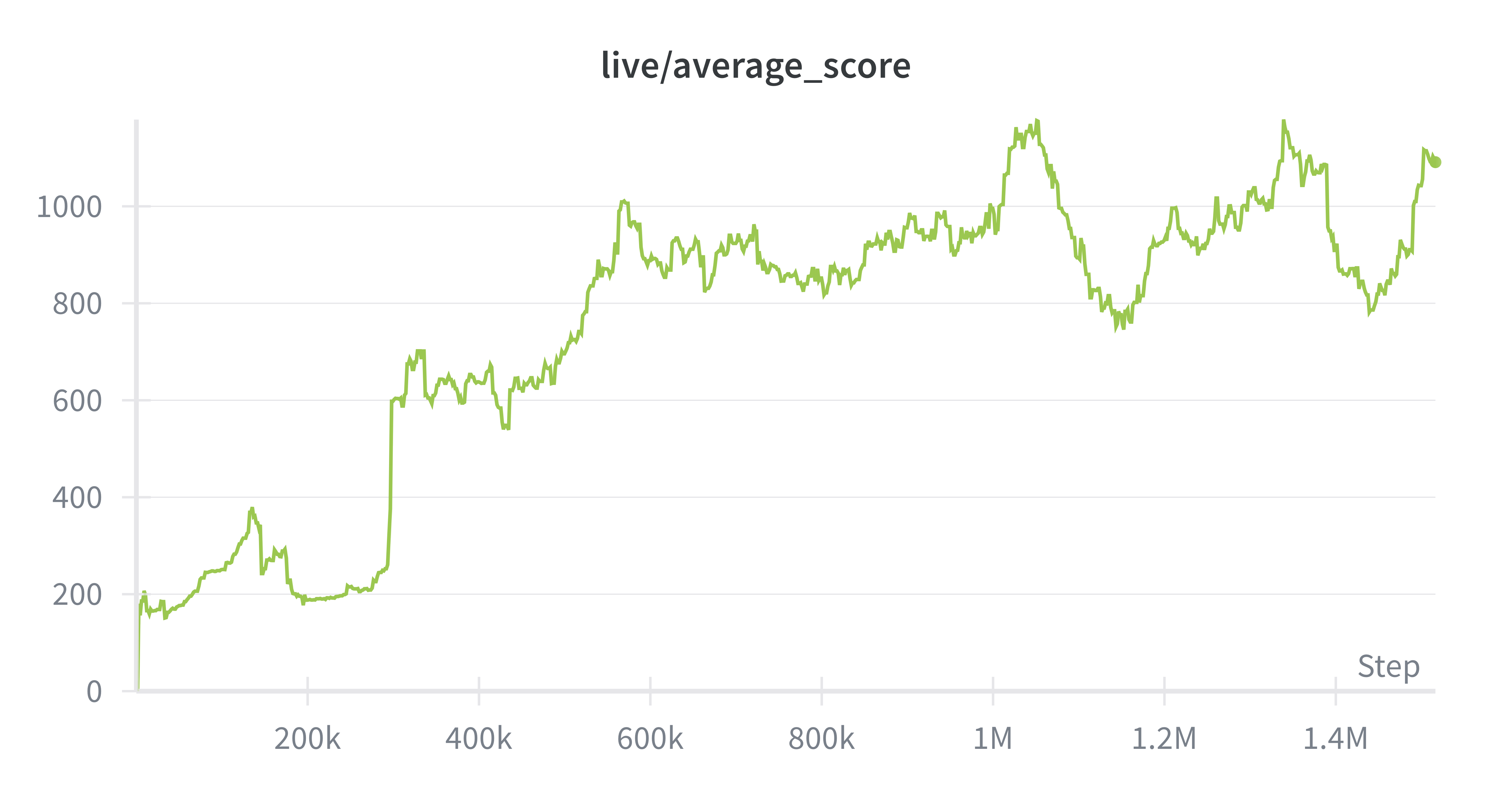
Delay Target was developed internally by engineers at Keen AGI, it is not an algorithm we've seen in any literature. In our experiments, agents trained with Delay Target significantly outperformed all other approaches. The original implementation is available in the Physical Atari repo.
Conceptually, Delay Target is closest to DQN augmented with CUDA graph–based optimizations and several additional techniques.
Key Features
Cached bootstrap targets instead of a target network
Rather than running a separate target model to compute bootstrap values, the agent stores its most recent value estimate for each visited transition in a state_value_buffer. When training, it forms targets by bootstrapping from these cached values which effectively introduces a lagged target without maintaining a separate target network. The benefit is that using a single network avoids the roughly 2x computational overhead of maintaining two networks, especially important on resource-constrained edge devices.
TD(λ)-style multi-step target blending
Targets are built from a mixture of multi-step discounted rewards plus discounted cached bootstrap values over a horizon up to multisteps_max. This is implemented via precomputed reward and value discount vectors, giving a smoother/less noisy target than pure 1-step TD.
Online + replay mixed minibatches
Each training batch contains a small online_batch of the most recent transitions (to keep learning tied to the current data/policy) plus additional samples from the replay/ring buffer (for diversity and reuse). Online samples can also be loss-scaled to emphasize fresh data.
Softmax-greedy action selection with adaptive temperature
Actions are chosen by sampling from a softmax over Q-values rather than ε-greedy. The temperature is tied to an EMA of recent prediction error (via avg_error_ema), so the policy explores more when uncertain and becomes greedier as the model stabilizes.
Observations
Compared to our spiky Rainbow DQN, Delay Target shows a steadier upward learning trend. This is likely because it uses more stable targets. Instead of constantly recomputing a fast-changing bootstrap target, it bootstraps from cached value estimates that update more slowly. This prevents the sudden drops and recoveries we see from regular DQN. Also the TD-lambda style multi-step targets smooth learning by combining information from several look-ahead lengths instead of relying on a single one-step backup. Together, these choices seem to reduce abrupt policy changes and produce a more monotonic improvement curve than Rainbow.
PPO
Proximal Policy Optimization (PPO) is a policy gradient method designed to promote stability by avoiding large policy updates. It's an on-policy algorithm, which means each piece of data in the current training batch must be computed from the current policy.
Key Features
On-Policy Policy Gradient
PPO is an on-policy algorithm, meaning all data used for gradient updates must be generated by the current policy. Experience becomes invalid once the policy is updated, which prevents reuse of off-policy data and tightly couples data collection to learning.
Actor–Critic Architecture
PPO uses an actor-critic formulation with a shared backbone and two output heads: a policy head that predicts a distribution over actions, and a value head that estimates the state value used for bootstrapped returns. The critic reduces variance in policy gradient estimates and stabilizes training.
Clipped Surrogate Objective
The core PPO update is governed by a clipped surrogate loss that constrains how much the policy can change in a single update. This constrains policy updates so that each new policy differs from the current policy by no more than the current policy differed from its predecessor.
Entropy Regularization
A fixed entropy bonus is added to the policy loss to encourage exploration by preventing premature collapse of the action distribution. This term decays in influence over training as the policy becomes more confident.
Generalized Advantage Estimation (GAE)
PPO typically uses GAE to compute low-variance, temporally-smoothed advantage estimates. This trades off bias and variance in the policy gradient and improves learning stability, especially in environments with delayed rewards.
Observations
PPO has proven to be extremely effective in producing good policies on Atari games, with the caveat that it is extremely data hungry, and doesn't use off-policy data. This means that it's much harder to get right on a physical setup than in simulation. In simulation there are some key advantages. One is that you can parallelize your environments, meaning each batch of data is less correlated sequentially (lower variance). The second is that you can “pause your environment” so while backprop is happening you aren't collecting off-policy data.
Running PPO out of the box is not viable
In a real-time setting, applying an on-policy algorithm presents two difficult options. Either learning must be parallelized across many robots to reduce sample variance, or policy updates must be deferred until episode completion. Our setup does not allow large-scale parallelism, and delaying updates until episode boundaries would severely limit the number of learning steps.
We initially attempted to train PPO with a small buffer size of 256 frames (~8 seconds of experience). However, during backpropagation the control loop was blocked, causing the agent to stop acting in the environment. This meant Ms. Pacman frequently died while learning updates were being computed, biasing the collected data toward states near the start of each episode.
At the same time, we also didn't want to only train once per episode (a whole day will only get you ~250 updates). So we split the agent into an actor-learner architecture. While the learner network performs gradient updates, a separate copy of the network continues interacting with the environment to prevent early death. The frames collected during this period are explicitly marked as off-policy. This allows for continuous data collection and prevents the replay buffer from being dominated by early-episode states, at the cost of losing a subset of frames that are off-policy.
Exploration collapses
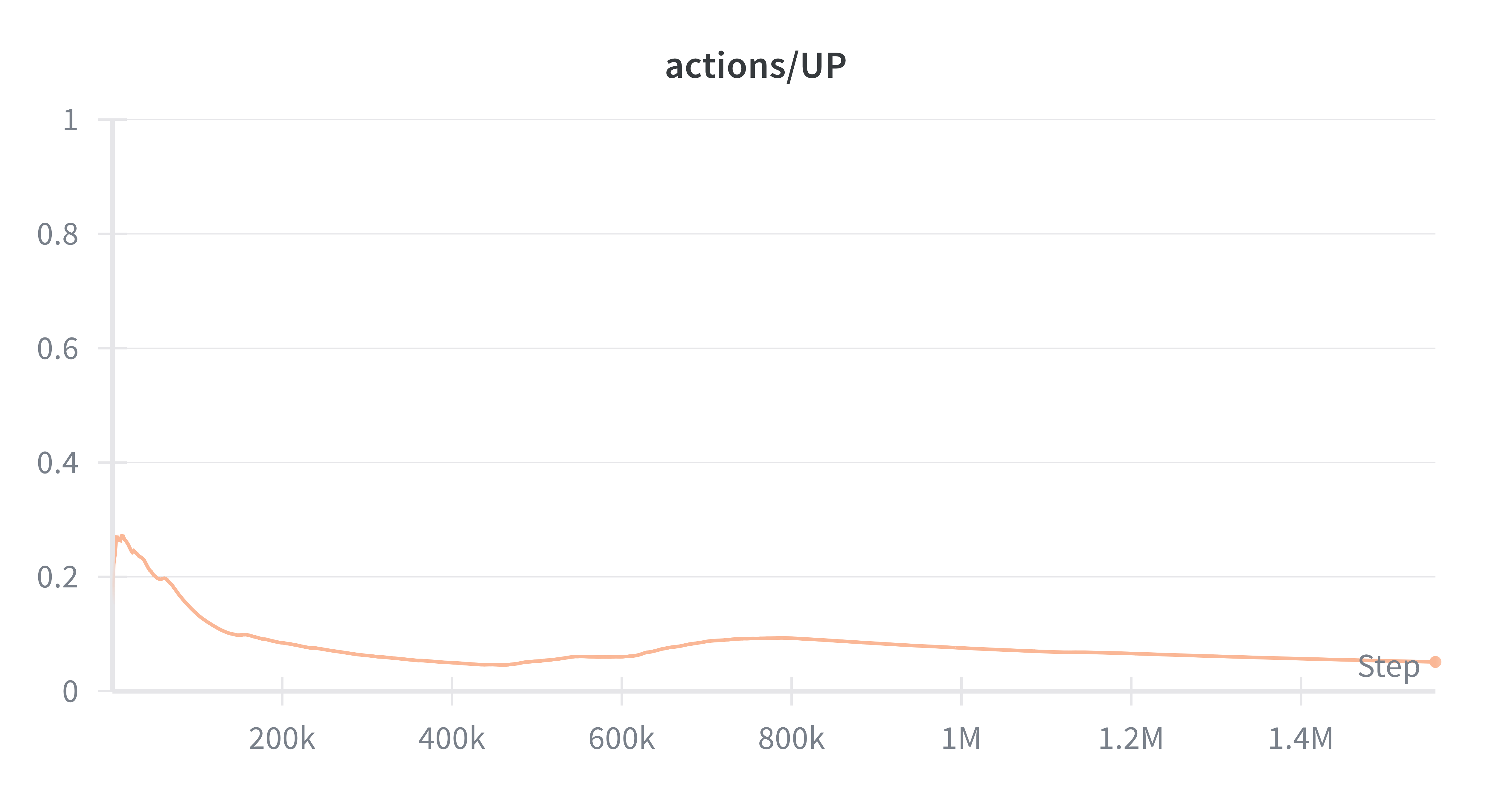
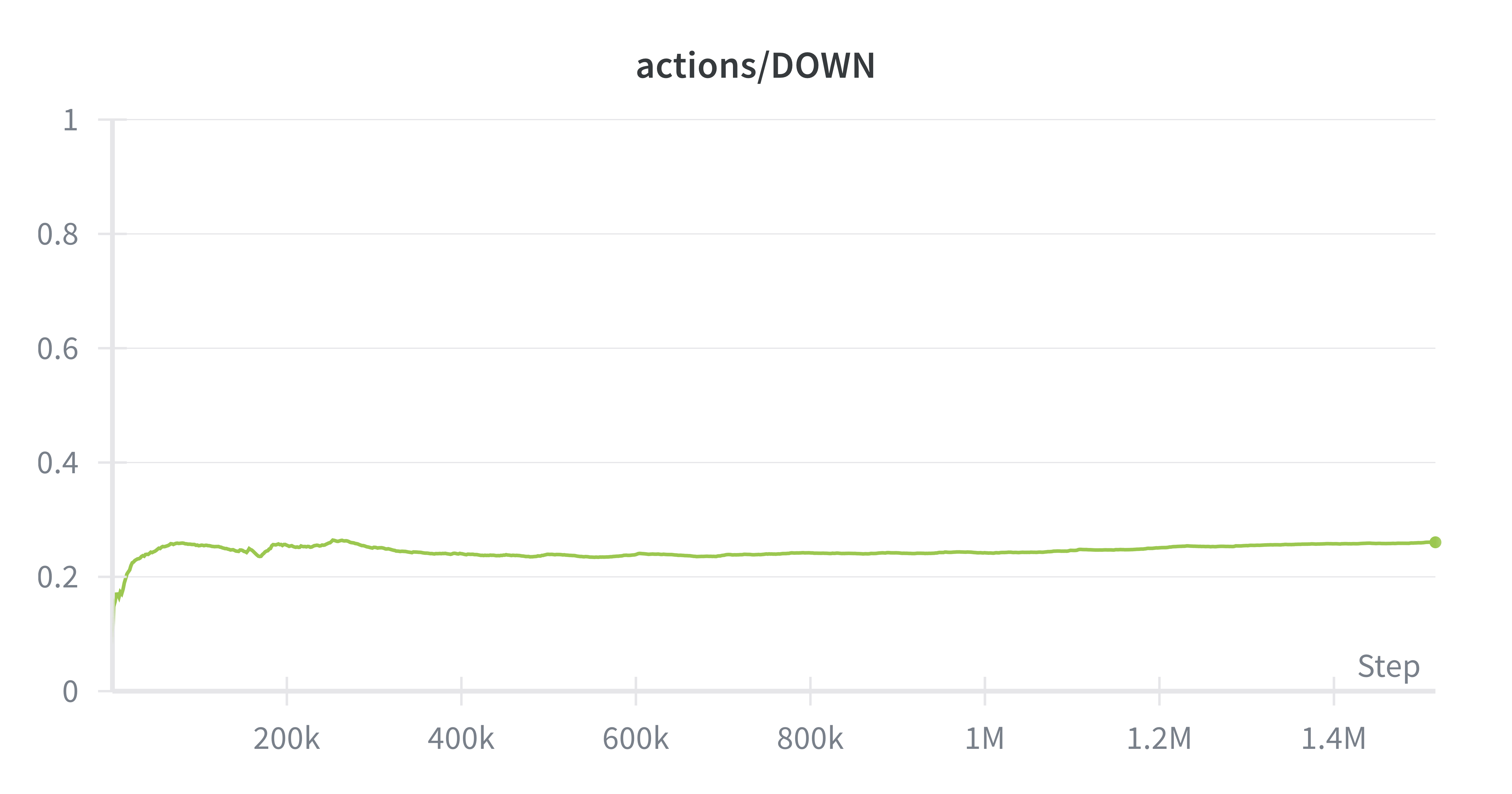
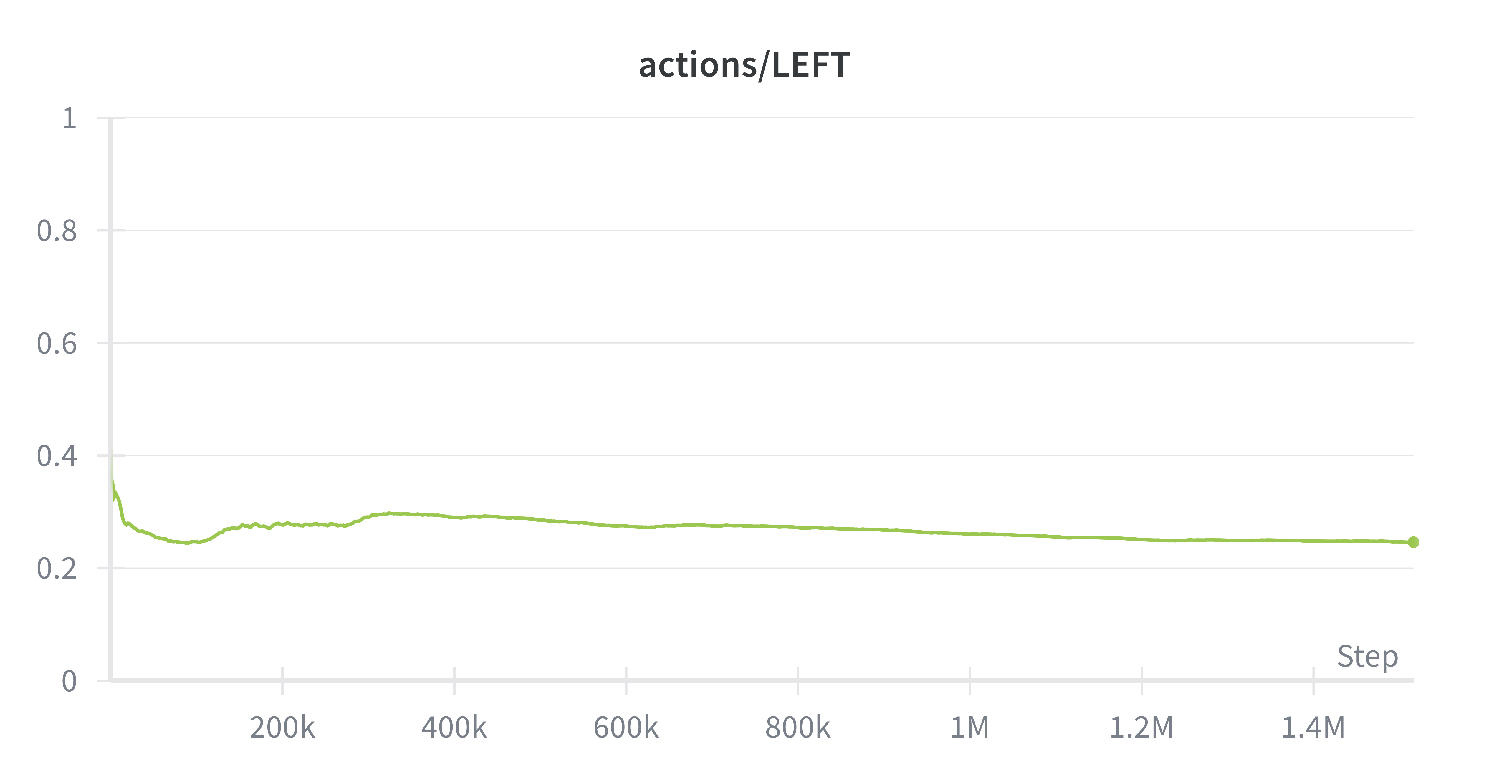
UP
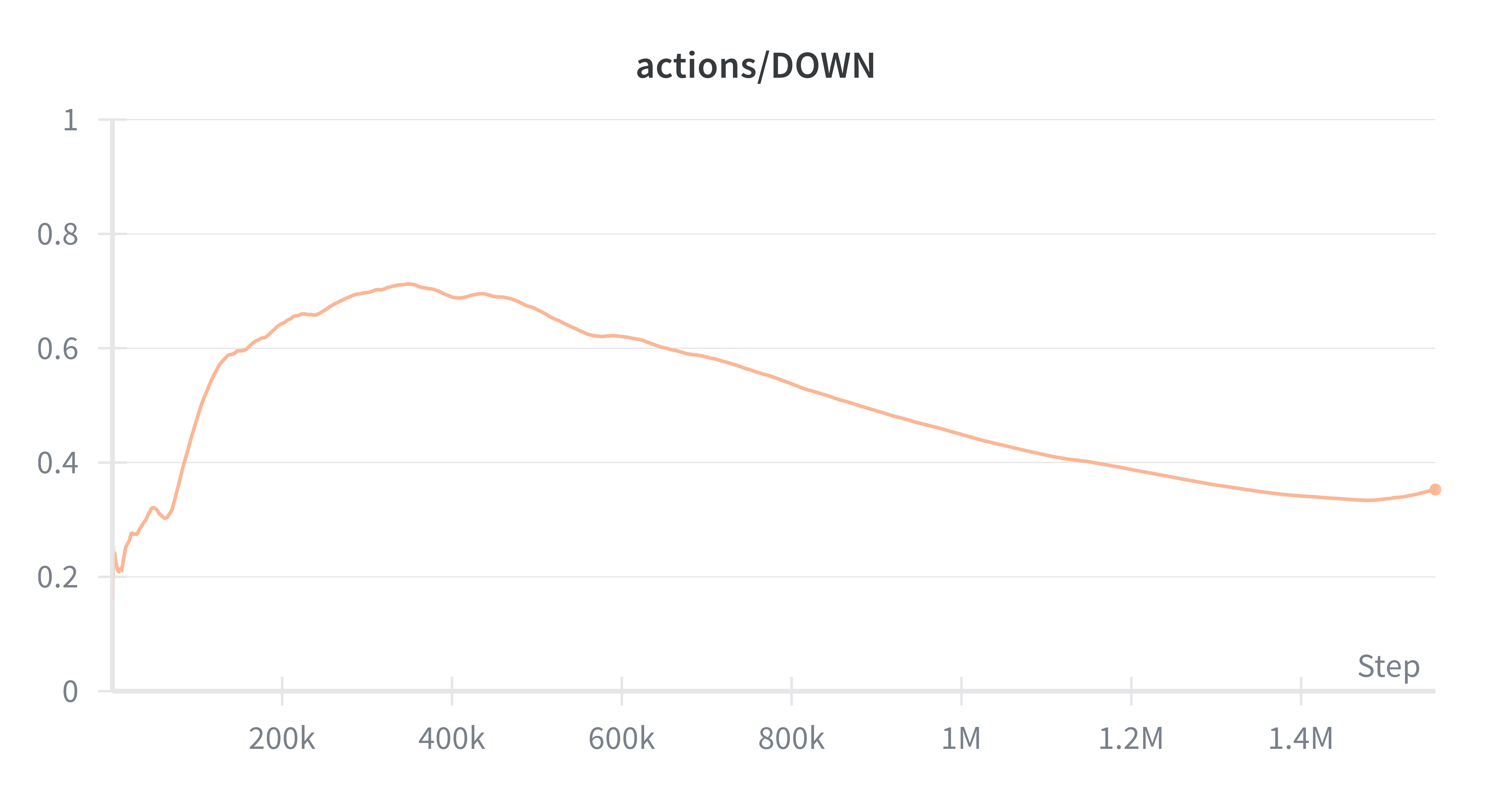
DOWN
LEFT
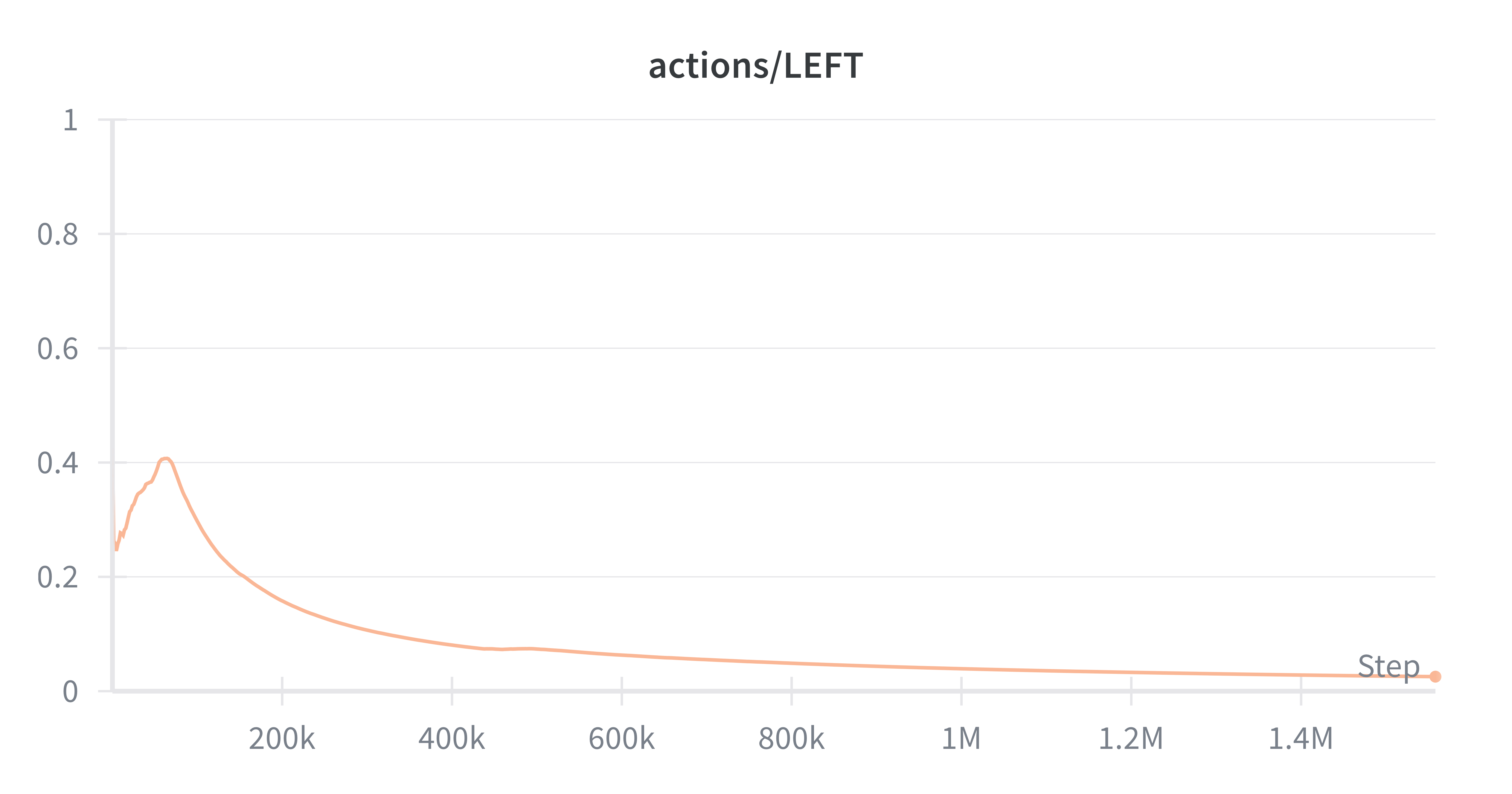
RIGHT
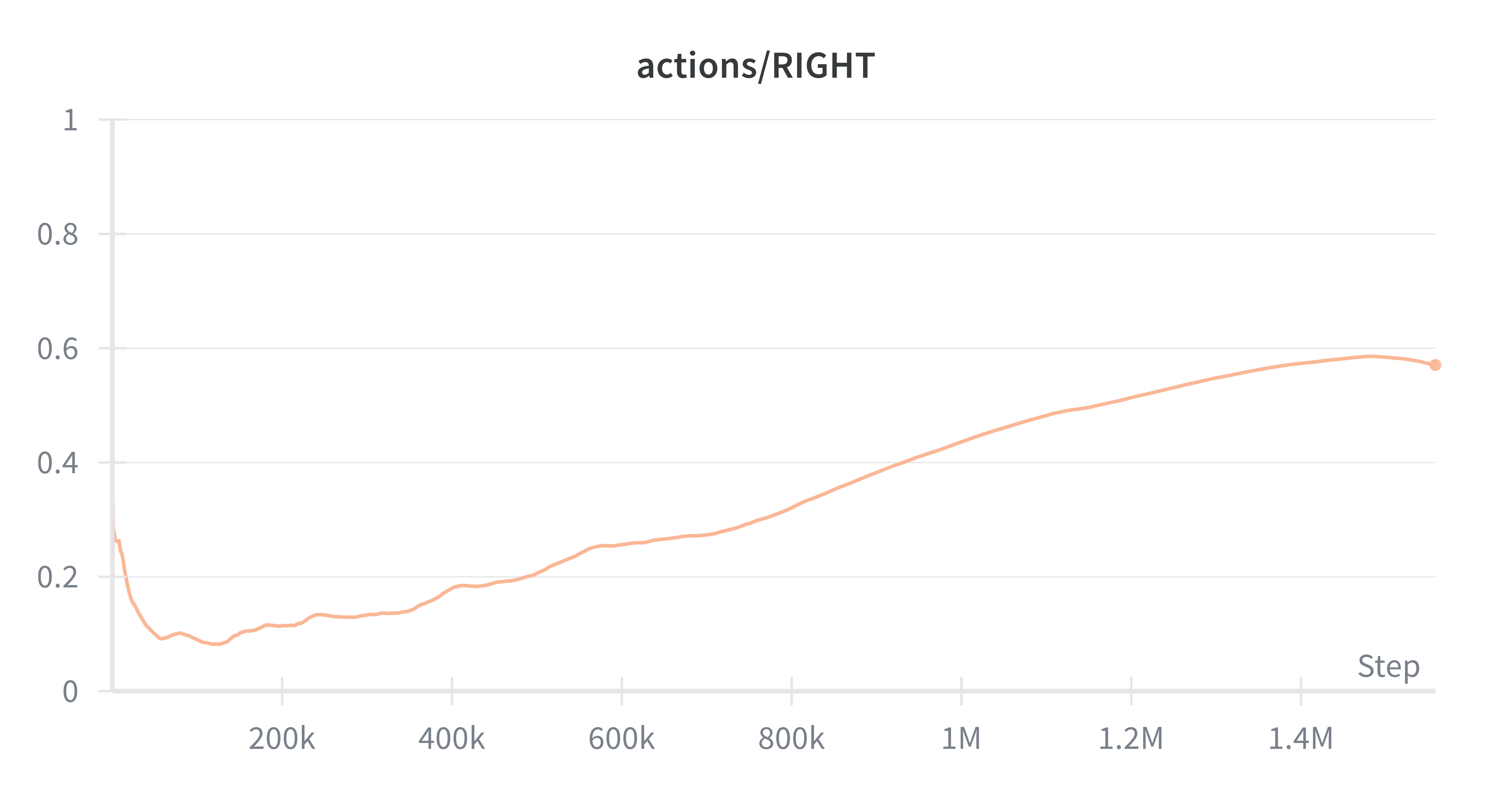
Since Ms. Pacman requires sustained exploration to avoid early local maxima, policy collapse can be deadly. With a theoretical ceiling of ~10k updates over 12 hours (at 60fps, 256-step buffers), our agent must be extremely efficient with each update. Our trials in simulation showed consistent scores of over 1k were only possible after about 1M steps, orders of magnitude beyond what our physical setup can handle.
PPO utilizes a fixed entropy bonus to reduce the likelihood of policy collapse. Unfortunately in ablations across learning rate, batch size, buffer sizes, and entropy decay steps, we were unable to find the right hyper parameter choices to ensure that our agent was learning while avoiding collapse. This is because 1) with a real robot hyperparameter searches are intractable because each experiment takes 12 hours and 2) physical environments are not reproducible.
In benchmarking PPO, we aim to show some of the limitations of policy gradient methods on real-time RL systems. The behavior that these policy gradient methods exhibit is they converge to a few actions at first, and rely on sampling often from policy in order to escape that local maxima. It was clear that PPO was underperforming other Q based methods, and we believe this was due to the data scale required for PPO agents to learn.
SAC
Soft-Actor-Critic (SAC) is an off-policy actor-critic algorithm based on the maximum entropy reinforcement learning framework. SAC leverages off-policy learning to optimize a stochastic policy balancing policy improvement with entropy regularization. Our implementation of Discrete SAC was inspired by Alireza Kazemipour and notes from OpenAI.
Key Features:
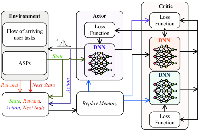
Off-Policy Actor-Critic
Combines Q-learning and policy gradient methods with both an actor network and a value network simultaneously independently updating based on bootstrapped targets.
Learned Entropy Coefficient
The entropy optimizer adjusts the entropy coefficient to promote continual exploration for the policy head, preventing early convergence.
Twin Q-Networks
Trains two separate Q networks, and during updates selects the min(Q1,Q2) in order to reduce overestimation of Q values.
Observations
UP
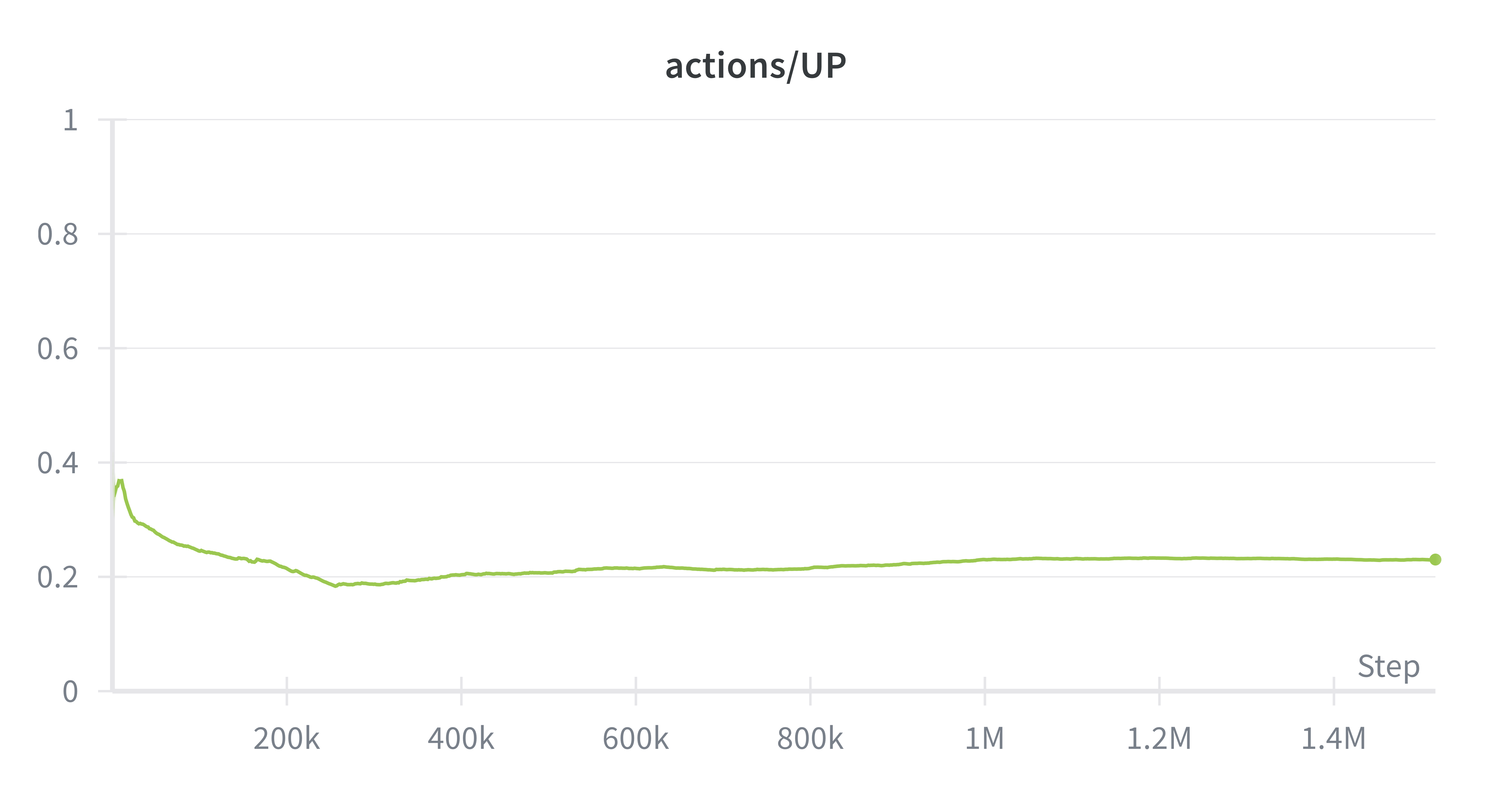
DOWN
LEFT
RIGHT

In training SAC on the physical atari, the main advantage we observed was the balancing of exploration against choosing optimal actions. Instead of converging to only two actions, SAC maintained a uniform distribution across actions, critical for Ms. Pacman. For example, our SAC agent was one of the few agents to travel through the wraparound.
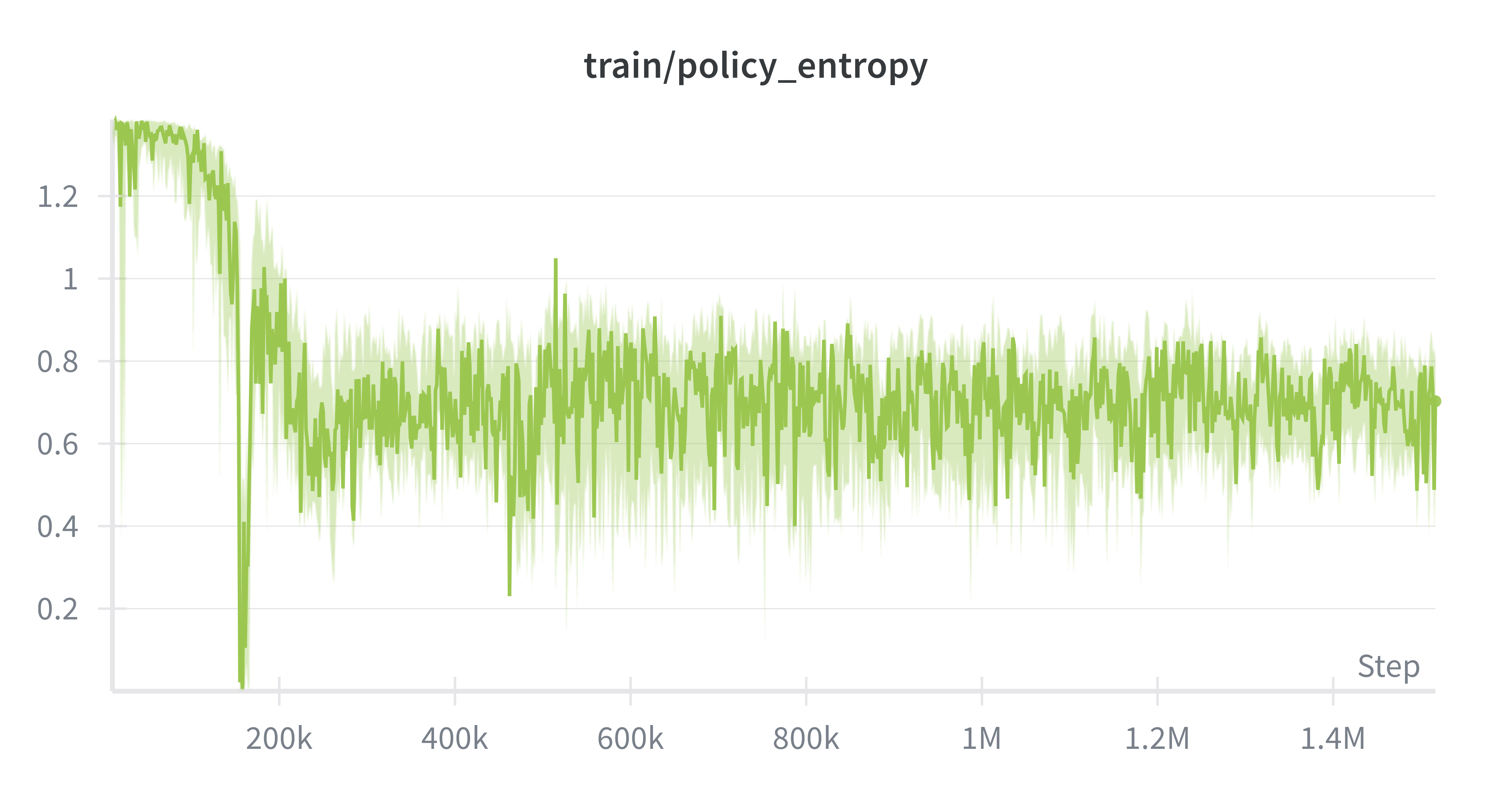
Ms. Pacman’s actions are constrained to 4 actions (up/down/left/right), so the maximum entropy in this system is ~1.3. Entropy regularization is forcing the policy output entropies to be around .67, which means that the policy doesn't get stuck often like PPO, while still being able to mostly take the correct action. We observed that SAC did not degenerate into just two actions (down/right), and was able to learn some interesting behaviors like ghost-chasing and power-up consumption.
Takeaways
Q-Learning vs Policy Gradient
A recurring theme in our experiments was the tension between sample efficiency and policy expressiveness. Q-learning methods were far more sample-efficient, while policy gradient methods produced more flexible behaviors.
Sample Efficiency
The efficiency gap stems from how each family uses experience. Q-learning stores transitions in a replay buffer and revisits them many times, extracting more learning signal per environment step. Policy gradient methods, by contrast, optimize the current policy using on-policy rollouts; once a batch is used for an update, it is discarded. In a regime where each environment step takes real time this difference is critical. Our PPO runs exhausted their update budget long before escaping initial collapse, while DQN variants continued improving throughout the session.
Policy Expressiveness
Policy gradient methods offer advantages in expressiveness. Because actions are sampled stochastically from a learned distribution, these policies can maintain uncertainty and avoid premature commitment. We observed this qualitatively: our SAC agent was one of the few to discover the wraparound tunnel, a strategy that requires sustained exploration away from pellet-dense regions.
Value-based methods, by contrast, are prone to locking onto high-variance strategies early in training. We observed DQN agents repeatedly chasing ghosts without a power pellet, a strategy that has huge rewards when it works but fails most of the time. After a few lucky ghost-eating sequences, the Q-values for “move toward ghost” spike, and the greedy policy repeats the behavior even when no pellet is active. The entropy-regularized policy gradient methods were better at hedging against these traps.
Action Smoothness
Stochastic policies also produce smoother control. During evaluation runs we could hear the difference: the joystick driven by DQN jerked back and forth between discrete directions, while SAC's probabilistic sampling created softer, more continuous motion. Whether this smoothness improves gameplay is unclear, but it may matter in domains where actuator wear or jerk constraints are relevant.
Future Directions - Continual Learning + Big World Hypothesis
In our experience with the Ms. Pacman robot-controller project, one of the most important findings was that sim-to-real transfer did not work. Across the algorithms we tried, policies that looked strong in simulation failed to transfer reliably to the physical setup, even after adding a latency wrapper intended to mimic controller dynamics during sim training. Our guess is the source of difficulty was not a single factor like delay, but a long tail of small mismatches introduced by the real system, including camera viewpoint, lighting and exposure, display artifacts, and controller timing jitter.
This observation aligns with the Big World Hypothesis as described by Javed & Sutton. The hypothesis says that in many decision-making problems the agent is orders of magnitude smaller than the environment. It must learn to make sound decisions using a limited understanding of the environment and limited resources. An opposing view is that many real-world problems have simple solutions and that sufficiently large, over-parameterized agents can discover those solutions and then act optimally in perpetuity. But in our case, even though the underlying game dynamics are fixed, the physical deployment seemed to create enough variation that a fixed policy learned in simulation was not robust. Although the physical setup is a small testbed, it's interesting that these issues arose.
A natural reaction to sim-to-real failure is to increase simulator fidelity. Better latency models, richer observation noise, and domain randomization can reduce the gap and are valuable tools for iteration. However, our experience suggests that higher-fidelity simulators are better viewed as a stepping stone rather than the final solution. Each improvement tends to expose additional sources of mismatch, and the physical system still contains variation that is difficult to account for in advance. In this framing, simulation is most useful for warm-starting policies, while robust performance depends on the ability to adapt to environments on the fly using continual learning.
Experimenting with continual learning on the Physical Atari testbed could lead to new algorithms that perform well in real world robotics. The testbed occupies a useful middle ground: it introduces real-world sensing and timing effects such as camera noise, lighting variation, and actuation delay, while remaining comparatively simple, repeatable, and easy to reset.